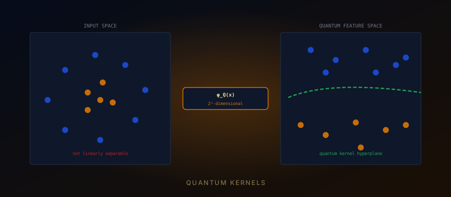
The kernel trick is one of the most elegant ideas in machine learning. Support vector machines find a separating hyperplane between two classes — but the hyperplane lives not in the original data space, where classes are often tangled together, but in a high-dimensional feature space reached by an explicit mapping . The kernel trick bypasses the need to compute at all: it only requires the inner product , which for many useful feature maps can be computed directly as a simple function of and . The feature space can be infinite-dimensional; the computation stays tractable.
Quantum computers introduce a new possibility. A quantum circuit acting on qubits maps classical data into a quantum state in a Hilbert space of dimension — exponentially large in the number of qubits. Inner products in this space, , are the transition amplitudes of quantum circuits and can be estimated by running on a quantum computer and measuring the probability of the all-zeros outcome. If this quantum inner product captures structure in the data that no efficiently computable classical kernel can, and if computing it classically is hard, there is a potential quantum advantage in machine learning.
Whether that potential translates into a practical advantage on any real dataset is the central open question in quantum kernel methods.
Key Concepts in This Article
Kernel Function
k(x, x') = ⟨φ(x), φ(x')⟩ — the inner product between feature maps of two data points. The kernel trick evaluates this without explicitly computing φ(x), making SVMs tractable even in infinite-dimensional feature spaces.
Quantum Feature Map
A parametrised quantum circuit U(x) that encodes classical data x as a quantum state |φ(x)⟩ = U(x)|0ⁿ⟩ in a 2ⁿ-dimensional Hilbert space. The quantum kernel is k_Q(x, x') = |⟨φ(x')|φ(x)⟩|².
Kernel Matrix
The n×n matrix K where Kᵢⱼ = k(xᵢ, xⱼ) over all training pairs. The SVM optimisation requires only K, not the individual feature vectors. For a quantum kernel, estimating K requires O(n²) quantum circuit executions.
Quantum Advantage Condition
Quantum kernel advantage requires two simultaneous conditions: the kernel must be hard to estimate classically, AND the data must have structure that the quantum kernel captures better than any efficiently computable classical kernel. Both are required.
Classical SVMs and the Kernel Trick
A support vector machine solves a binary classification task by finding the maximum-margin hyperplane separating two classes. When data is not linearly separable in the input space ℝᵈ, the kernel trick allows SVMs to operate in a much richer feature space without the computational cost of explicitly computing the feature vectors.
The SVM dual problem depends only on the kernel matrix entries : it never requires the feature vectors explicitly. Once the kernel matrix is computed, the SVM optimisation is a classical quadratic programme — convex, efficiently solvable, and well-understood theoretically.
The power of the kernel trick is that for the polynomial kernel of degree 2, for instance, implicitly computes inner products in a feature space of dimension without ever constructing a -dimensional vector. For the RBF kernel, the feature space is infinite-dimensional.
Quantum Feature Maps: Encoding Data Into Hilbert Space
A quantum feature map is a parametrised quantum circuit U(x) that encodes classical data x ∈ ℝᵈ as a quantum state:
The resulting state lives in a 2ⁿ-dimensional Hilbert space. For n = 20 qubits, this is over a million dimensions; for n = 50, it is a quadrillion. The appeal is obvious — and the danger is equally obvious, as we will see.
The key design principle for quantum feature maps is non-linearity through entanglement. Single-qubit rotations alone (Rz(xᵢ) on qubit i) encode each feature independently — the resulting kernel is separable and can be computed efficiently classically. The entangling layers (ZZ interactions between qubit pairs) introduce correlations between features: the circuit encodes not just xᵢ but products like xᵢxⱼ, (xᵢ)²(xⱼ), and higher-order terms in the amplitudes. With L layers of such interactions, the feature map encodes polynomials of degree up to L·n in the original features — an exponentially rich function class.
Evaluating the Quantum Kernel
The elegance of this evaluation is that no ancilla qubits or SWAP tests are required. The circuit U†(x’)U(x) acting on |0ⁿ⟩ prepares a state whose all-zeros projection is exactly the desired inner product. Running this circuit T times and counting |0ⁿ⟩ outcomes estimates the kernel entry with statistical error O(1/√T).
Once the kernel matrix K is fully estimated — requiring O(n²) such circuits for n training points — a classical SVM solver minimises the dual objective:
subject to and , where are class labels and is the regularisation parameter. This is a standard quadratic programme solved by well-established classical software. The quantum contribution is entirely in the kernel matrix entries; the learning is classical.
New test points are classified by computing for each support vector and evaluating the sign of . This again requires quantum kernel evaluations per test point.
The Rigorous Quantum Advantage: Liu et al. 2021
In 2021, Yunchao Liu, Srinivasa Raghu, and colleagues published a paper in Nature Physics that provided the first rigorous, unconditional quantum advantage for a supervised learning task using quantum kernels.
The key construction: they defined a classification problem based on a variant of the discrete logarithm problem — a problem related to Simon’s algorithm and Shor’s algorithm. They proved two things simultaneously:
-
Classical hardness: any classical machine learning algorithm (not just SVMs) requires an exponential number of training samples to learn the classification with better than random accuracy, assuming the learning with errors (LWE) hardness conjecture.
-
Quantum efficiency: a quantum kernel SVM using the appropriate quantum feature map learns the same classification task with a polynomial number of training samples.
This is a genuine, unconditional quantum advantage for machine learning — the quantum algorithm solves a learning problem that classical algorithms cannot, under well-established cryptographic assumptions.
The critical qualification: the learning problem is artificial. It is constructed to have quantum structure by design — its hardness for classical learners comes directly from a cryptographic assumption, and the quantum advantage arises because the feature map is essentially implementing a quantum algorithm that breaks the underlying hardness. No natural real-world dataset has this structure.
The Hilbert Space Trap: More Dimensions Are Not Always Better
In the same year, Huang, Broughton, Cotler, and colleagues published a complementary negative result in Nature Communications: for generic datasets, quantum models do not outperform classical kernel methods, and the key predictor of advantage is the alignment between the quantum kernel and the data structure — not the dimensionality of the feature space.
The central theorem: if a quantum kernel k_Q(x, x’) can be approximated efficiently classically — even if the quantum feature space is exponentially large — then a classical SVM with that approximated kernel achieves the same classification accuracy. The exponential Hilbert space only provides advantage if it contains structure that is simultaneously:
- Hard to access classically (the kernel circuit cannot be efficiently simulated)
- Genuinely predictive for the target classification task
The problem: random quantum circuits satisfy condition 1 (they are hard to simulate classically for large n) but not condition 2 (their output has no particular alignment with the structure of real datasets — images, tabular data, time series). A high-dimensional feature space that is random with respect to your data is not useful; it is noise.
This is the Hilbert space trap: the temptation to assume that more dimensions automatically yield better classification. Classical kernels like the RBF kernel work well on most datasets precisely because they are designed with geometric intuition about what distances mean for natural data. Quantum feature maps, designed for their classical hardness rather than their geometric relevance, often perform no better than or worse than RBF SVMs on standard benchmarks.
Quantum vs Classical: When Does the Quantum Kernel Win?
The Computational Cost Problem
Quantum kernel SVMs face a practical overhead that is easy to overlook. For n training points:
- Kernel matrix: O(n²) quantum circuit executions, each taking T shots for precision. For n=1000 training samples and T=1000 shots per kernel entry: 10⁹ circuit executions.
- Classical SVM: the quadratic programme scales as O(n² d) or O(n³) for the kernel version — but with n=1000 and d=100 features, this is 10⁷ floating-point operations.
- Test prediction: each new test point requires O(|SVs|) quantum circuit evaluations — not a one-time cost.
Classical RBF and polynomial kernels compute each kernel entry in O(d) floating-point operations. For d=100 and n=1000: 10⁸ classical operations for the full matrix — still much cheaper per entry than quantum circuit execution plus measurement.
This overhead means quantum kernel SVMs are currently slower than classical SVMs even for problems where the quantum kernel is theoretically better. The crossover — where the quantum kernel’s higher accuracy justifies the overhead — requires either datasets where classical kernels fail fundamentally (as in Liu et al.’s constructed problem) or quantum hardware fast enough to close the circuit execution gap.
What Has Actually Been Demonstrated
Havlíček et al. (2019) demonstrated quantum kernel classification and a linear classification method (quantum variational classifier) on a 2-qubit IBM processor using an artificially constructed dataset that was designed to be separable by the quantum kernel but not by a linear classical classifier. The demonstration showed the algorithm works on real hardware; it did not demonstrate advantage over classical SVM with a classical kernel on a real-world problem.
Subsequent benchmarks on standard datasets — UCI repository, financial data, molecular properties — have consistently found that classical kernel methods (RBF SVM, gradient boosting, neural networks) match or outperform quantum kernel SVMs. The quantum kernel sometimes achieves competitive accuracy, but the training costs are substantially higher and the accuracy advantage is not systematic.
One area with genuine promise: quantum data. When the data being classified is the output of quantum simulations — measurement outcomes from quantum circuits, molecular electronic states, or other quantum-mechanical systems — a quantum feature map is a natural choice, and classical feature maps may struggle to represent the relevant quantum structure efficiently. This niche does not exist on today’s classical datasets but becomes relevant as quantum computers are used as scientific instruments generating quantum data for analysis.
The Honest Assessment
Quantum kernel SVMs occupy an interesting theoretical position: the Liu et al. result proves that quantum machine learning advantage exists — the question is not whether quantum kernels can outperform classical learning, but whether they do so on problems that matter.
The field needs one of two things to progress. Either a dataset arising from a natural scientific or engineering problem where quantum structure genuinely drives hardness for classical methods — and where quantum kernels provably or empirically provide better generalisation. Or a theoretical argument that some class of practically important problems has the algebraic structure needed for quantum advantage.
What the field currently has: a rigorous proof of existence for an artificial problem, competitive-but-not-superior performance on real datasets, and an exponentially large feature space that is expensive to use and often no better than a carefully tuned RBF kernel.
That is a genuine scientific result. It is not yet a practical advantage. The difference matters, and the quantum machine learning community has become increasingly candid about it — which is itself a sign of a maturing field.
Sources & Further Reading
- Supervised Learning with Quantum-Enhanced Feature Spaces. Nature 567, 209; arXiv:1804.11326 (2019)
- Quantum Machine Learning in Feature Hilbert Spaces. Physical Review Letters 122, 040504; arXiv:1803.07128 (2019)
- A Rigorous and Robust Quantum Speed-Up in Supervised Machine Learning. Nature Physics 17, 1013; arXiv:2010.02174 (2021)
- Power of Data in Quantum Machine Learning. Nature Communications 12, 2631; arXiv:2011.01938 (2021)
Discussion